
Introduction
Most data-science tutorials make outlier detection look trivial: drop everything beyond three standard deviations and move on. On real datasets — where distributions are skewed and a stakeholder asks why a particular point was removed — that simplicity falls apart. To probe the problem, an experiment tested five of the most commonly used outlier-detection methods on a single real dataset of 6,497 Portuguese wines to ask a basic question: do these methods agree? They did not, and the disagreements turned out to be more instructive than any textbook rule.

The dataset
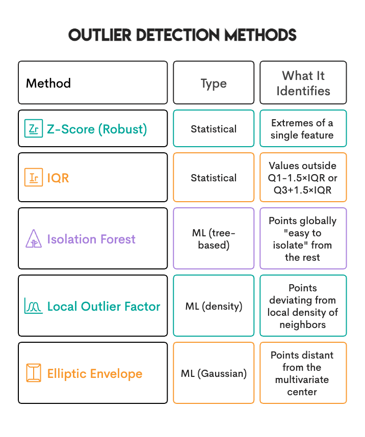
The data is the wine-quality dataset, publicly available through the UCI Machine Learning Repository. It contains physicochemical measurements for 6,497 Portuguese “vinho verde” wines (1,599 red and 4,898 white), along with quality ratings from expert tasters. It was chosen because it is real production data rather than synthetic; its distributions are skewed (6 of 11 features have skewness greater than 1), so it violates textbook assumptions; and the quality ratings make it possible to check whether detected “outliers” cluster among unusually rated wines. The five methods tested are listed below.
A first surprise: the cost of testing many features
Before the methods could be compared, a problem appeared. With 11 features, the naive approach — flagging a sample if any single feature is extreme — produced badly inflated results. The IQR method labeled roughly 23% of the wines as outliers, and the per-feature error rate compounds quickly across many features.

A more conservative rule flags a sample only when at least two features are simultaneously extreme. Here is the improved version:
# Count extreme features per sample
outlier_counts = (np.abs(z_scores) > 3.5).sum(axis=1)
outliers = outlier_counts >= 2
Comparing five methods on one dataset
With the methods implemented, the next step counted how many samples each one flagged.

The machine-learning methods were set up as follows:
from sklearn.ensemble import IsolationForest
from sklearn.neighbors import LocalOutlierFactor

iforest = IsolationForest(contamination=0.05, random_state=42)
lof = LocalOutlierFactor(n_neighbors=20, contamination=0.05)
Real differences: the methods find different things
Across the 6,497 wines, only 32 samples (0.5%) were flagged by all four primary methods, and 143 samples (2.2%) were identified by three or more. The rest were flagged by only one or two methods. This is not a bug; it reflects that each method defines “abnormal” differently.

If a wine has far higher residual sugar than average, that is a global outlier and methods such as the Z-score or IQR will catch it. But if that wine sits among other wines with similar sugar levels, a local method like LOF will not flag it, because it is normal in its local context. The useful question is therefore not “which method is best?” but “what kind of unusual am I looking for?”
Sanity check: are outliers tied to wine quality?
Because the dataset includes expert quality ratings (3 to 9), it was possible to ask whether flagged outliers appear more often among certain ratings.
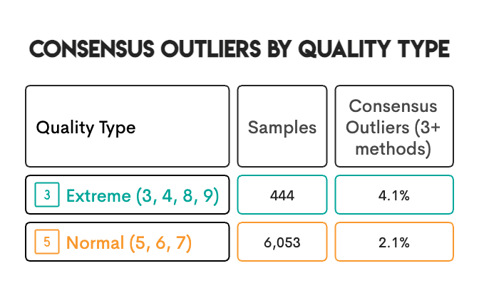
Highly rated wines were about twice as likely to be unanimous outliers, which is a reassuring sanity check: unusual physicochemical profiles can correspond to genuinely distinctive, high-quality wines rather than errors.
Three decisions that shaped the results
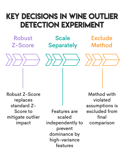
Several methodological choices materially changed the outcome.
# Robust Z-Score using median and MAD
median = np.median(data, axis=0)
mad = np.median(np.abs(data - median), axis=0)
robust_z = 0.6745 * (data - median) / mad
First, a robust Z-score was used instead of the standard Z-score. The standard version relies on the mean and standard deviation, both of which are themselves distorted by outliers; the robust version uses the median and median absolute deviation (MAD), which are not. As a result, the standard Z-score flagged 0.8% of the data while the robust Z-score flagged 3.5%. Second, red and white wines were scaled separately, since the two types have different baseline levels; the interquartile range was computed within each wine type and then combined.
# Scale each wine type separately
from sklearn.preprocessing import RobustScaler
scaled_parts = ()
for wine_type in ('red', 'white'):
    subset = df(df('type') == wine_type)(features)
    scaled_parts.append(RobustScaler().fit_transform(subset))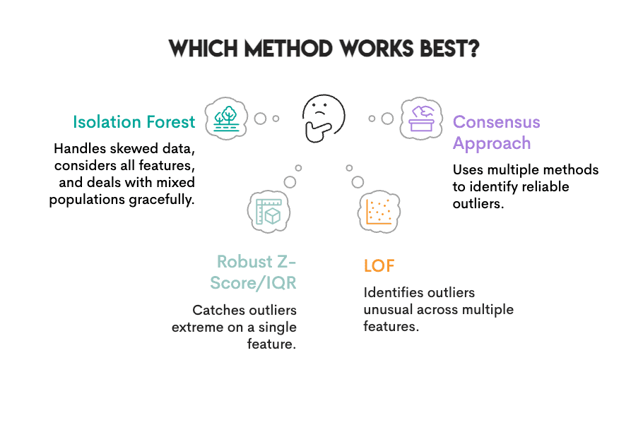
Which method performs best for this dataset?
Given the data’s heterogeneity, mixed populations, and lack of known ground truth, the robust Z-score, IQR, Isolation Forest, and LOF all handle skewed data reasonably well. If a single method had to be chosen, Isolation Forest is a sensible default: it makes no distributional assumptions, considers all features at once, and behaves acceptably with mixed populations. But no single method does everything — Isolation Forest can miss points that are extreme on only one feature, while the Z-score and IQR can miss points that are unusual across several features at once. The stronger approach is to use multiple methods and rely on consensus: the 143 wines flagged by three or more methods are far more trustworthy than anything flagged by one method alone.
# Count how many methods flagged each sample
consensus = zscore_out + iqr_out + iforest_out + lof_out
high_confidence = df(consensus >= 3)  # Identified by 3+ methods
Without ground truth, which is the norm in real projects, agreement between methods is the closest available measure of confidence.
What this means for your own projects
A few practical principles follow. Define the problem before choosing a method: data-entry errors, measurement issues, and genuine rare cases all look different and call for different tools. Check assumptions, because heavily skewed data will mislead the standard Z-score and the elliptic envelope, so the distribution should be examined first. And use multiple methods, treating samples flagged by three or more different definitions of “outlier” as more reliable than those flagged by one.
Concluding remarks
The lesson is not that outlier detection is broken but that “outlier” means different things to different methods. The Z-score and IQR capture values that are extreme on a single dimension; Isolation Forest and LOF surface points that stand out in the overall pattern; and the elliptic envelope works well only when the data is genuinely Gaussian, which this dataset was not. The right starting point is to decide exactly what kind of unusual matters, and when that is unclear, to run several methods and compare.
Common questions
Which technique should come first? Isolation Forest is a reasonable default, since it ignores the data’s distribution and uses all features together. To flag extreme values on one specific measurement, the Z-score or IQR may be more appropriate. How should the contamination rate be chosen for scikit-learn methods? It depends on the problem; 5% (0.05) is a common starting value, but it is an assumption about how many outliers exist rather than a measured fact, so it should be revisited against the data and the goal.
