
Introduction
Whereas data preprocessing While data holds substantial relevance in science and machine learning workflows, these processes are often not conducted correctly, largely because they require overly complex, time-consuming, or extensive custom code. As a result, practitioners may delay essential tasks such as data cleansing, rely on brittle ad-hoc solutions that are not sustainable in the long run, or over-engineer solutions to problems that may be simple at their core.
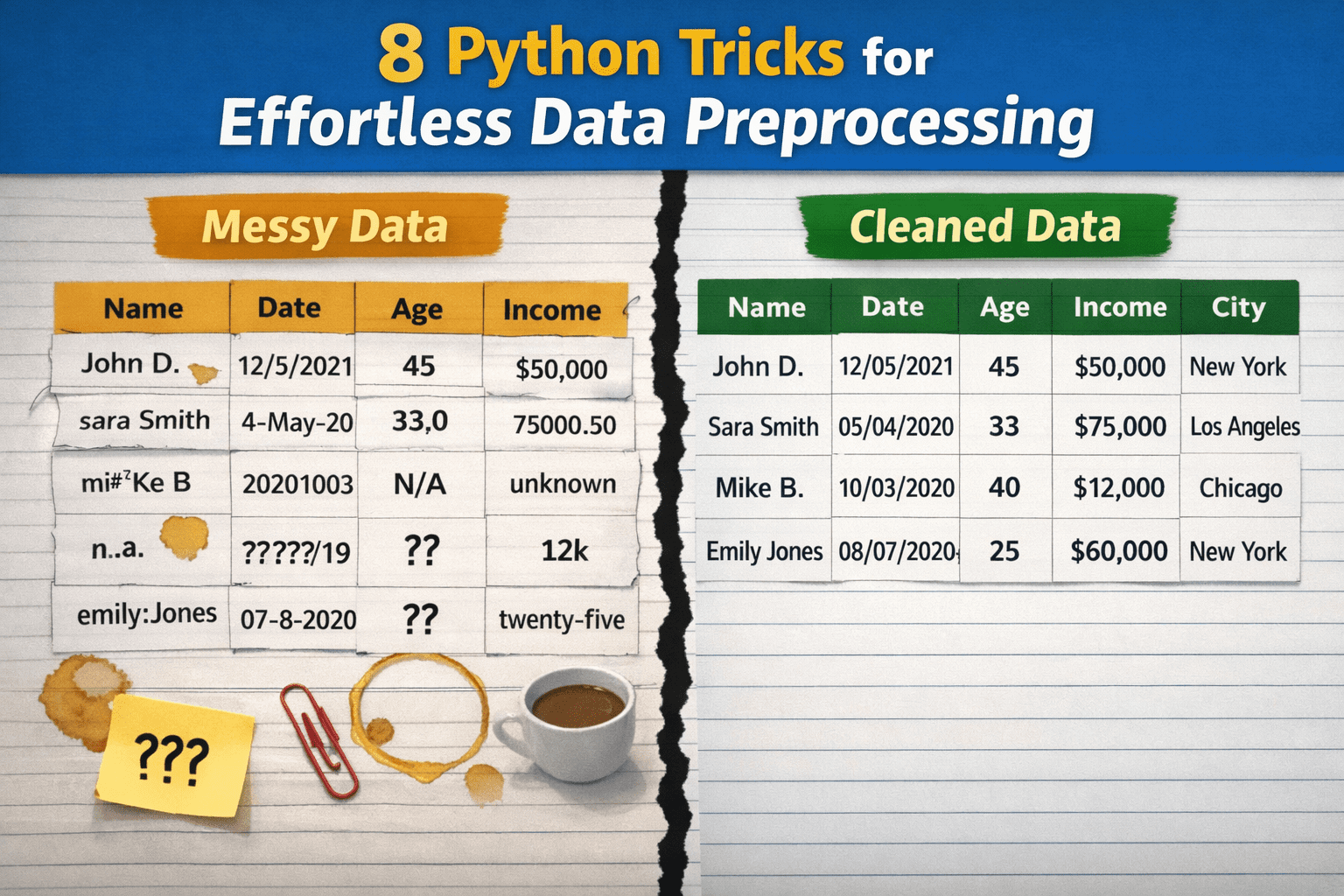
This article presents 8 Python tricks to transform raw, dirty data into clean, neat pre-processed data with minimal effort.
Before looking at specific tricks and related code examples, the following introduction code sets up the necessary libraries and defines a toy dataset to illustrate each trick:
import pandas as pd
import numpy as np
# A tiny, intentionally messy dataset
df = pd.DataFrame({
    " User Name ": (" Alice ", "bob", "Bob", "alice", None),
    "Age": ("25", "30", "?", "120", "28"),
    "Income$": ("50000", "60000", None, "1000000", "55000"),
    "Join Date": ("2023-01-01", "01/15/2023", "not a date", None, "2023-02-01"),
    "City": ("New York", "new york ", "NYC", "New York", "nyc"),
})
1. Quickly normalize column names
This is a very useful, one-liner style trick: in one line of code, it normalizes the names of all columns in the dataset. The specifics depend on how the attribute names should be normalized, but the following example shows how to replace whitespace with underscore symbols and lowercase everything, ensuring a consistent, standardized naming convention. This is important to prevent annoying bugs or fix potential typos in downstream tasks. No need to repeat column by column!
df.columns = df.columns.str.strip().str.lower().str.replace(" ", "_")2. Separating whitespace from strings at scale
Sometimes junk that is invisible to the human eye, such as spaces at the beginning or end of string (categorical) values, needs to be systematically removed across the entire dataset. This strategy does this neatly for all columns containing strings, leaving other columns such as numeric values unchanged.
df = df.apply(lambda s: s.str.strip() if s.dtype == "object" else s)3. Converting numeric columns safely
When it is not certain that all values in a numeric column follow the same format, it is usually a good idea to explicitly convert these values into a numeric format, which can sometimes turn a jumbled string of numbers that looks like numbers into real numbers. In a single line, this replaces what would otherwise require try/except blocks and a more manual cleaning process.
df("age") = pd.to_numeric(df("age"), errors="coerce")
df("income$") = pd.to_numeric(df("income$"), errors="coerce")
Note here that other classical approaches like df('columna').astype(float) Sometimes a crash may occur if invalid raw values are found that cannot be trivially converted to numeric.
4. Parsing Dates errors="coerce"
Same validation-oriented process, specific data types. This trick converts date-time values that are valid, discarding those that are not. using the errors="coerce" is the key to tell Panda If invalid, non-convertible values are found, they should be converted NaT (not time), instead of generating an error during execution and crashing the program.
df("join_date") = pd.to_datetime(df("join_date"), errors="coerce")5. Fixing Missing Values with Smart Defaults
For those who are unfamiliar with strategies for handling missing values other than deleting entire rows, this strategy imputes those values – filling in the gaps – like using statistical-driven defaults. median Or mode. An efficient, one-liner-based strategy that can be adjusted with different default sets. (0) The index that comes with the mode is used to obtain only one value in case of relationships between two or several “most frequent values”.
df("age") = df("age").fillna(df("age").median())
df("city") = df("city").fillna(df("city").mode()(0))
6. Standardizing Categories with Maps
In hierarchical columns with diverse values such as cities, it is also necessary to standardize the names and remove possible anomalies to obtain clean group names and create downstream group aggregation. groupby() Reliable and effective. With the help of a dictionary, this example applies a one-to-one mapping to string values corresponding to New York City, ensuring that they are all represented identically by “NYC”.
city_map = {"new york": "NYC", "nyc": "NYC"}
df("city") = df("city").str.lower().map(city_map).fillna(df("city"))
7. Removing duplicates intelligently and flexibly
The key to this highly customizable duplicate removal strategy is to use subset=("user_name"). In this example, it is used to tell Pandas to treat a row as a duplicate just by looking at it. "user_name" Column, and verifying whether the value in the column is the same as the value in the other row. This is a great way to ensure that each unique user is represented only once in the dataset, preventing double counting, and all in one instruction.
df = df.drop_duplicates(subset=("user_name"))8. Shredding volumes for external removal
The final trick involves automatically capping extreme values or outliers rather than removing them altogether. For example, particularly useful when outliers are considered to be caused by errors manually introduced into the data. Clipping sets the extreme values falling below (and above) two percentiles (1 and 99 in the example) with such percentile values that the original values remain unchanged between the two specified percentiles. In simple words, it is like keeping extremely large or small values within limits.
q_low, q_high = df("income$").quantile((0.01, 0.99))
df("income$") = df("income$").clip(q_low, q_high)
Limitations and What to Watch
These tricks make common preprocessing steps faster, but each carries trade-offs worth remembering. Automatic type conversion and outlier clipping change data, so it is wise to inspect what was altered rather than trusting a one-liner blindly — coercing bad values to missing, or capping at the 1st and 99th percentiles, can hide real problems or discard legitimate extremes. Filling missing values with defaults introduces assumptions that can bias later analysis, and aggressive de-duplication can merge records that only look identical. Category mappings need maintenance as new values appear. In short, these are conveniences for well-understood data, not substitutes for understanding the dataset; validating results after each step remains essential. Full behavior and edge cases are documented in the pandas documentation. Clean inputs also improve model accuracy downstream, as shown in these XGBoost tuning tricks for forecasting.
Wrapping Up
This article describes eight useful tips, tricks, and strategies that will strengthen data preprocessing pipelines in Python, making them more efficient, effective, and robust: all at the same time.
