

Interviews at Meta, Apple, Amazon, Netflix and Alphabet — collectively known as FAANG — rarely test whether a candidate can recite textbook definitions. They are designed to reveal whether a candidate analyses data critically and can catch a flawed analysis before it reaches production. A reliable way to probe that skill is to present common statistical traps: a dashboard figure that looks fine but is misleading, or an experiment result that seems actionable but hides a structural flaw.
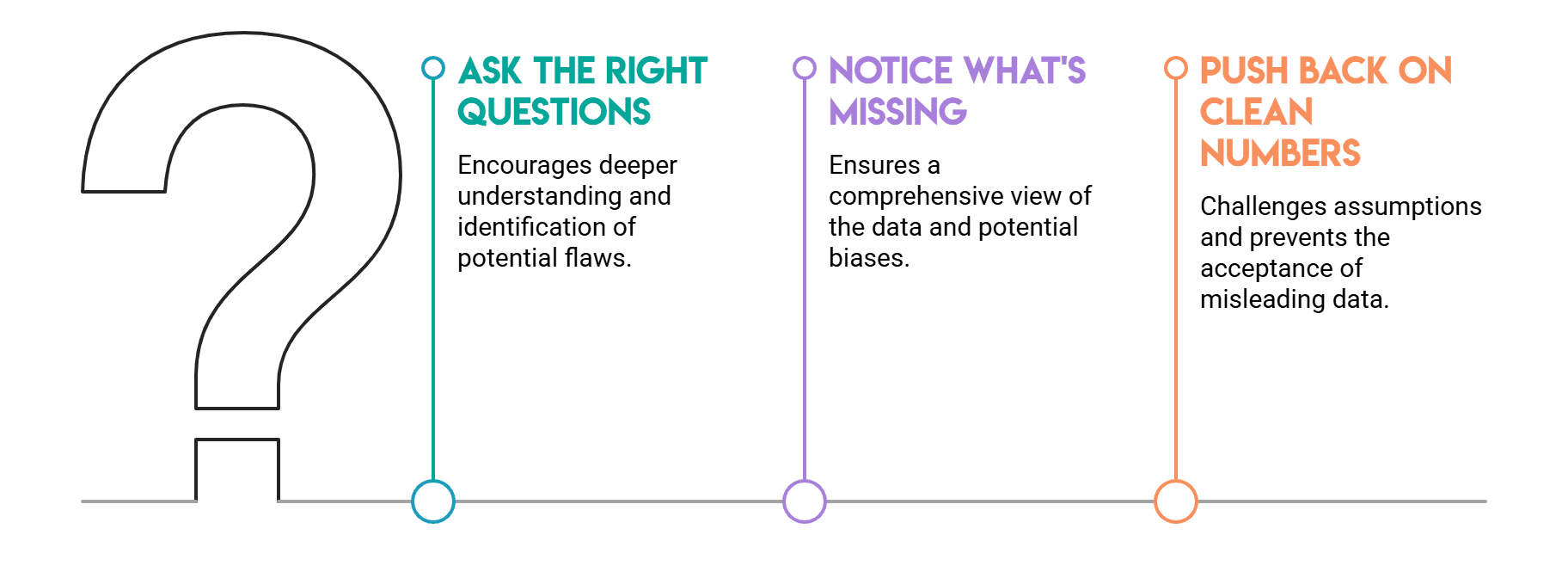
These scenarios mirror everyday decisions analysts face. The interviewer usually knows the answer already; what they are assessing is the candidate’s thought process — whether the right questions get asked, whether missing information is noticed, and whether numbers that look good at first glance are treated with appropriate caution. Strong mathematical backgrounds are no guarantee against these traps. The five below are among the most frequently tested.
Simpson’s Paradox
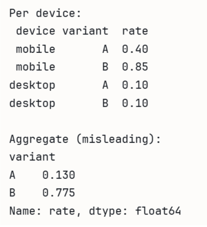
Simpson’s Paradox occurs when a trend that appears in aggregated data reverses once the data is split into meaningful subgroups. A treatment or variant can look better overall while being worse within every individual segment, because group sizes and base rates distort the combined figure. In a product setting, an A/B test that reports only the overall conversion rate can point in exactly the wrong direction. The recommended habit is to segment before drawing conclusions, and to be wary of any headline rate that aggregates dissimilar groups.
Performance with A/B test data
The following demonstration uses pandas to show how an aggregate rate can mislead.
import pandas as pd

# A wins on both devices individually, but B wins in aggregate
# because B gets most traffic from higher-converting mobile.
data = pd.DataFrame({
    'device':   ('mobile', 'mobile', 'desktop', 'desktop'),
    'variant':  ('A', 'B', 'A', 'B'),
    'converts': (40, 765, 90, 10),
    'visitors': (100, 900, 900, 100),
})
data('rate') = data('converts') / data('visitors')

print('Per device:')
print(data(('device', 'variant', 'rate')).to_string(index=False))
print('nAggregate (misleading):')
agg = data.groupby('variant')(('converts', 'visitors')).sum()
agg('rate') = agg('converts') / agg('visitors')
print(agg('rate'))
The output is shown below:
Selection Bias
This trap assesses whether a candidate considers where data comes from before analysing it. Selection bias arises when the available data is not representative of the population of interest. Because the bias lives in the collection process rather than the analysis, it is easy to miss. A common interview frame is a survey finding that 80% of users are satisfied: a strong answer notes that satisfied users are more likely to respond, so the figure probably overstates true satisfaction because dissatisfied users opt out. Similar reasoning applies to churned customers, where the sample is conditioned on an outcome.
Simulating survey non-response
A short simulation makes the effect of non-response concrete.
import numpy as np
import pandas as pd

np.random.seed(42)
# Simulate users where satisfied users are more likely to respond
satisfaction = np.random.choice((0, 1), size=1000, p=(0.5, 0.5))
# Response probability: 80% for satisfied, 20% for unsatisfied
response_prob = np.where(satisfaction == 1, 0.8, 0.2)
responded = np.random.rand(1000) < response_prob

print(f"True satisfaction rate: {satisfaction.mean():.2%}")
print(f"Survey satisfaction rate: {satisfaction(responded).mean():.2%}")
The output is shown below:

P-Hacking
P-hacking refers to running many analyses, or repeatedly testing, until something crosses the conventional significance threshold — then reporting only that result. With enough comparisons, false positives are almost guaranteed. Interviewers look for awareness that searching across many cuts of the data inflates the chance of a spurious “significant” finding, and that pre-registration of hypotheses and metrics is the standard defence.
Watching false positives accumulate
The simulation below shows how false positives accumulate as the number of tests grows.
import numpy as np
from scipy import stats
np.random.seed(0)

# 20 A/B tests where the null hypothesis is TRUE (no real effect)
n_tests, alpha = 20, 0.05
false_positives = 0

for _ in range(n_tests):
    a = np.random.normal(0, 1, 1000)
    b = np.random.normal(0, 1, 1000)  # identical distribution!
    if stats.ttest_ind(a, b).pvalue < alpha:
        false_positives += 1

print(f'Tests run:                 {n_tests}')
print(f'False positives (p<0.05): {false_positives}')
print(f'Expected by chance alone: {n_tests * alpha:.0f}')
The output is shown below:

Correcting for Multiple Testing
When many metrics are evaluated at once, the significance threshold needs adjustment. The Bonferroni correction is conservative and controls the chance of any false positive, at the cost of statistical power; the Benjamini–Hochberg procedure is more appropriate when some false discoveries are acceptable in exchange for greater power. A typical interview prompt — “we monitor 50 metrics per experiment; how do you decide which matter?” — is best answered by pre-specifying primary metrics before the experiment and treating secondary metrics as exploratory, while explicitly acknowledging the multiple-testing problem. The underlying point is that running more tests adds noise, not necessarily information.
Confounding Variables
This trap catches candidates who treat correlation as causation without asking what else might explain a relationship. A confounding variable influences both the independent and dependent variables, creating the illusion of a direct link where none exists. The expected response is to ask what third factor could be driving both quantities, and to consider controls, stratification or a randomised design before claiming a causal effect.
Simulating a spurious relationship
The example below constructs a confounded relationship to illustrate the point.
import numpy as np
import pandas as pd
np.random.seed(42)
n = 1000
# Confounder: user quality (0 = low, 1 = high)
user_quality = np.random.binomial(1, 0.5, n)
# App opens driven by user quality, not independent
app_opens = user_quality * 5 + np.random.normal(0, 1, n)
# Revenue also driven by user quality, not app opens
revenue = user_quality * 100 + np.random.normal(0, 10, n)
df = pd.DataFrame({
    'user_quality': user_quality,
    'app_opens': app_opens,
    'revenue': revenue
})
# Naive correlation looks strong — misleading
naive_corr = df('app_opens').corr(df('revenue'))
# Within-group correlation (controlling for confounder) is near zero
corr_low  = df(df('user_quality')==0)('app_opens').corr(df(df('user_quality')==0)('revenue'))
corr_high = df(df('user_quality')==1)('app_opens').corr(df(df('user_quality')==1)('revenue'))
print(f"Naive correlation (app opens vs revenue): {naive_corr:.2f}")
print(f"Correlation controlling for user quality:")
print(f"  Low-quality users:  {corr_low:.2f}")
print(f"  High-quality users: {corr_high:.2f}")
The output is shown below:
Naive correlation (app opens vs revenue): 0.91

Correlation controlling for user quality:

Low-quality users:  0.03
High-quality users: -0.07
Wrapping up
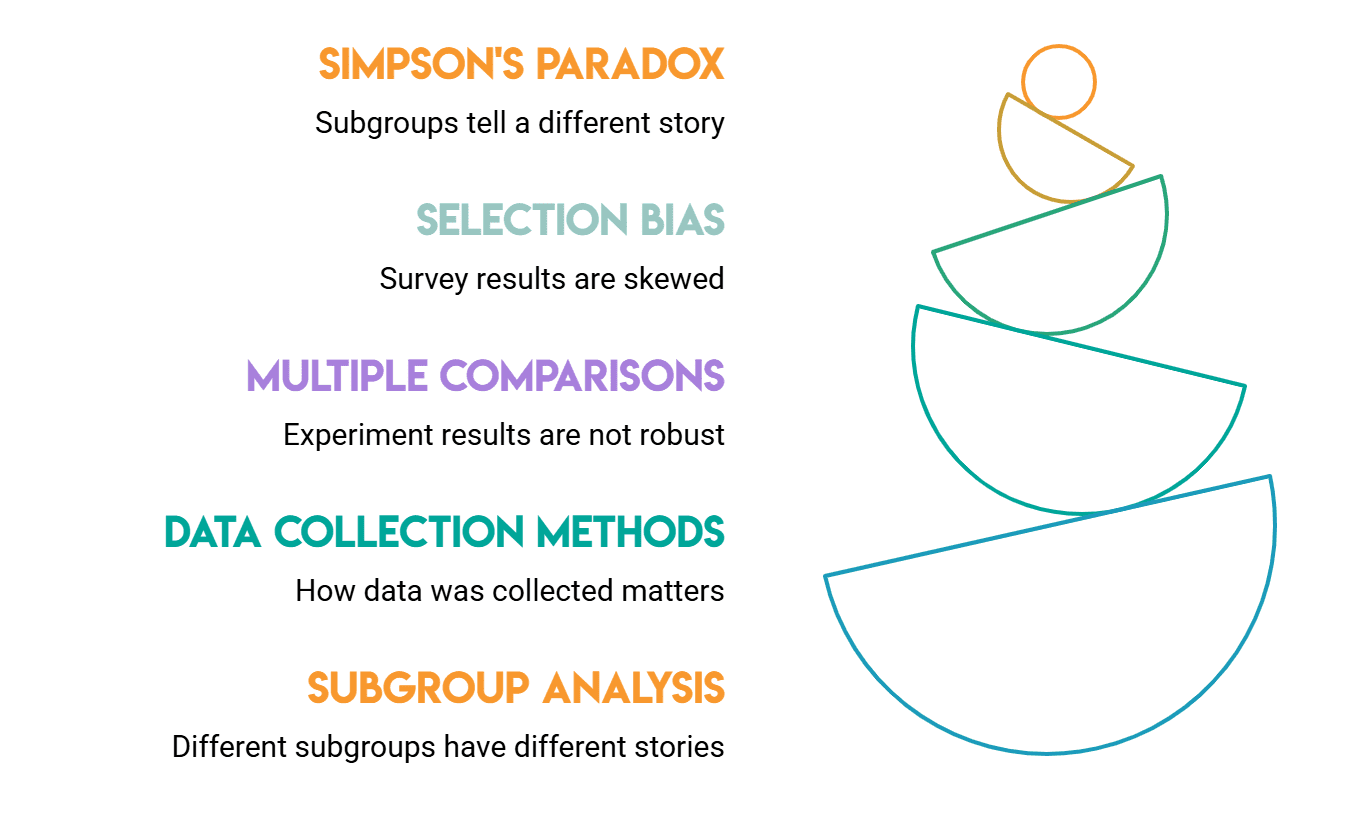
None of these ideas are conceptually difficult; interviewers ask about them because they are common failure modes in real data work. A candidate who spots Simpson’s paradox in a product metric, catches selection bias in a survey, or asks whether an experimental result survives multiple comparisons will make fewer poor decisions. Going into a FAANG interview, simply being disciplined about a few questions — How was this data collected? Are there subgroups that tell a different story? How many tests contributed to this result? — already puts a candidate ahead of most. Beyond interviews, these habits help keep flawed conclusions out of production.
One caveat worth keeping in mind: the code examples here are illustrative simulations meant to build intuition, not production-grade statistical tooling, and real datasets introduce complications these toy examples do not capture. A clear reference for several of these pitfalls is the overview of Simpson’s paradox.
