

Introduction
A keyword search often returns results that match the words in a query but miss its meaning, while a good recommendation engine can surface something highly relevant that was never explicitly requested. The gap between finding an exact word and understanding what someone actually meant is what makes a search feature genuinely useful. Vector search closes that gap by representing text as points in a high-dimensional space, where geometric proximity encodes semantic similarity. Two sentences can share no words at all and still sit close together because a model has learned that their meanings are related.
This tutorial builds a vector search engine from scratch using only Python and NumPy, so each step is visible: how embeddings are stored and normalised, why cosine similarity reduces to a dot product, and what the resulting search space looks like when projected into two dimensions.
What is vector search?
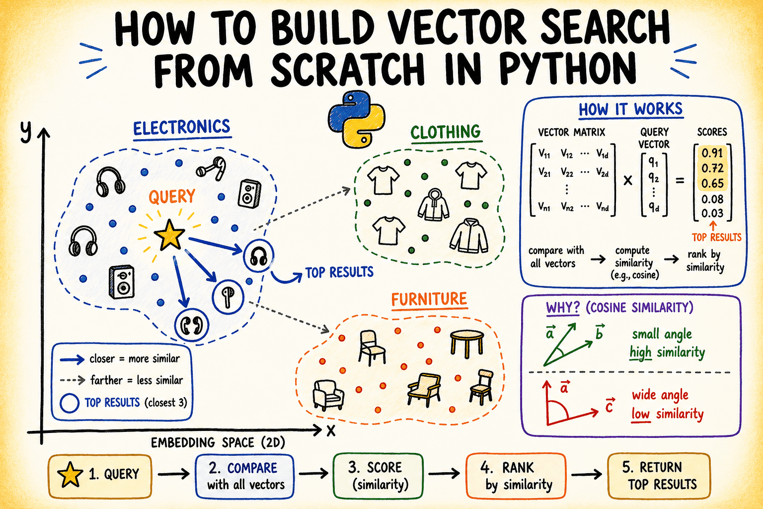
Traditional keyword search finds exact word matches. Vector search works differently: it converts documents and queries into numerical vectors called embeddings, then finds the vectors that lie closest together in a high-dimensional space. The key idea is that proximity in vector space corresponds to semantic similarity, so two passages that mean the same thing tend to have embeddings near one another.
The distance metric used to measure that proximity shapes the whole system. The most common choice is cosine similarity, which measures the angle between two vectors rather than their absolute distance. This makes it scale-invariant, which is useful when direction or meaning matters more than magnitude or word count.
Setting up the dataset
The example works with a small set of concise product descriptions from a hypothetical e-commerce catalogue, pre-embedded as low-dimensional vectors that are sufficient to demonstrate the concepts. In a real system these embeddings would be produced by a sentence-embedding model; here the step is simulated with controlled random data that has a clear cluster structure.
import numpy as np

np.random.seed(42)

# Product catalog — 3 semantic clusters: electronics, clothing, furniture
products = (
    "Wireless noise-cancelling headphones with 30-hour battery",
    "Bluetooth speaker with waterproof design",
    "USB-C hub with 7 ports and power delivery",
    "4K HDMI cable 6ft braided",
    "Mechanical keyboard with RGB backlight",
    "Men's slim-fit chino pants navy blue",
    "Women's merino wool turtleneck sweater",
    "Unisex running jacket lightweight windbreaker",
    "Leather chelsea boots for men",
    "Organic cotton crew neck t-shirt",
    "Solid oak dining table seats 6",
    "Ergonomic mesh office chair lumbar support",
    "Linen sofa 3-seater natural beige",
    "Bamboo bookshelf 5-tier adjustable",
    "Memory foam mattress queen size medium firm",
)

# Simulate embeddings with cluster structure
# Cluster centers in 8D space
electronics_center = np.array((0.9, 0.1, 0.2, 0.8, 0.1, 0.3, 0.7, 0.2))
clothing_center    = np.array((0.1, 0.8, 0.7, 0.1, 0.9, 0.2, 0.1, 0.8))
furniture_center   = np.array((0.2, 0.3, 0.9, 0.2, 0.1, 0.9, 0.3, 0.1))

n_per_cluster = 5
noise = 0.08

embeddings = np.vstack((
    electronics_center + np.random.randn(n_per_cluster, 8) * noise,
    clothing_center    + np.random.randn(n_per_cluster, 8) * noise,
    furniture_center   + np.random.randn(n_per_cluster, 8) * noise,
))

print(f"Embeddings shape: {embeddings.shape}")
Output:
Embeddings shape: (15, 8)Each row is a product and each column a dimension of its embedding. The product names are never used during search — only the embedding values matter.
Creating the index
An index in a vector search engine is simply a stored set of normalised embeddings. Normalisation matters because, once vectors are unit length, cosine similarity becomes equivalent to a dot product, which is cheaper to compute.
def normalize(vectors: np.ndarray) -> np.ndarray:
    """L2-normalize each row vector."""
    norms = np.linalg.norm(vectors, axis=1, keepdims=True)
    # Avoid division by zero
    norms = np.where(norms == 0, 1e-10, norms)
    return vectors / norms

class VectorIndex:
    def __init__(self):
        self.vectors = None
        self.labels = None

    def add(self, vectors: np.ndarray, labels: list):
        self.vectors = normalize(vectors)
        self.labels = labels
        print(f"Indexed {len(labels)} items with {vectors.shape(1)}-dimensional embeddings.")

    def search(self, query_vector: np.ndarray, top_k: int = 3):
        query_norm = normalize(query_vector.reshape(1, -1))
        # Cosine similarity = dot product of normalized vectors
        scores = self.vectors @ query_norm.T  # shape: (n_items, 1)
        scores = scores.flatten()
        # Get top-k indices sorted by descending score
        top_indices = np.argsort(scores)(::-1)(:top_k)
        return ((self.labels(i), float(scores(i))) for i in top_indices)

index = VectorIndex()
index.add(embeddings, products)
Output:
Indexed 15 items with 8-dimensional embeddings.The search method does three things: it normalises the query, computes dot products against every stored vector, then sorts by score and returns the top-k results. A single matrix multiplication of the stored vectors against the normalised query is the entire retrieval step.
Running queries
The engine can then be tested with a few queries. Query vectors are constructed by starting from one of the cluster centres and adding a little noise, simulating the kind of embedding a real query would produce.
def make_query(center: np.ndarray, noise_scale: float = 0.05) -> np.ndarray:
    return center + np.random.randn(8) * noise_scale


queries = {
    "audio equipment": make_query(electronics_center),
    "casual wear":     make_query(clothing_center),
    "home furniture":  make_query(furniture_center),
}

for query_name, q_vec in queries.items():
    print(f"\nQuery: '{query_name}'")
    results = index.search(q_vec, top_k=3)
    for rank, (label, score) in enumerate(results, 1):
        print(f"  {rank}. ({score:.4f}) {label}")
Output:
Query: 'audio equipment'
  1. (0.9856) Wireless noise-cancelling headphones with 30-hour battery
  2. (0.9840) USB-C hub with 7 ports and power delivery
  3. (0.9829) Mechanical keyboard with RGB backlight

Query: 'casual wear'
  1. (0.9960) Men's slim-fit chino pants navy blue
  2. (0.9958) Leather chelsea boots for men
  3. (0.9916) Women's merino wool turtleneck sweater

Query: 'home furniture'
  1. (0.9929) Bamboo bookshelf 5-tier adjustable
  2. (0.9902) Linen sofa 3-seater natural beige
  3. (0.9881) Solid oak dining table seats 6
Scores close to 1.0 indicate near-identical direction in the embedding space, which is exactly what is expected for queries built from the same cluster.
Visualising the embedding space
It helps to reason visually about high-dimensional data. Principal Component Analysis (PCA) projects the embeddings down to two dimensions so the cluster structure becomes visible; a minimal PCA can be implemented using only NumPy. The first block computes the 2D projection and plots all product embeddings with labels and cluster colours.
import matplotlib.pyplot as plt
import matplotlib.patches as mpatches

projected = pca_2d(embeddings)

cluster_colors = (
    ("#4A90D9") * 5 +   # electronics — blue
    ("#E8734A") * 5 +   # clothing — orange
    ("#5BAD72") * 5     # furniture — green
)
cluster_labels = ("Electronics") * 5 + ("Clothing") * 5 + ("Furniture") * 5

fig, ax = plt.subplots(figsize=(6, 4))
ax.scatter(projected(:, 0), projected(:, 1),
           c=cluster_colors, s=100, edgecolors="white", linewidths=0.7, zorder=3)
The next block projects the query vectors into the same space, overlays them and finalises the plot.
# Plot query projections
q_projected = pca_2d(
    np.vstack(list(queries.values())) - embeddings.mean(axis=0)
)
for (qname, _), (qx, qy) in zip(queries.items(), q_projected):
    ax.scatter(qx, qy, marker="*", s=200, color="gold",
               edgecolors="#333", linewidths=0.6, zorder=4)
    ax.annotate(f"⟵ query: {qname}", (qx, qy),
                textcoords="offset points", xytext=(6, -8),
                fontsize=7, color="#555555", style="italic")

legend_patches = (
    mpatches.Patch(color="#4A90D9", label="Electronics"),
    mpatches.Patch(color="#E8734A", label="Clothing"),
    mpatches.Patch(color="#5BAD72", label="Furniture"),
    mpatches.Patch(color="gold",    label="Query vectors"),
)
ax.legend(handles=legend_patches, loc="upper left", fontsize=6)
ax.set_title("Vector Search — Embedding Space (PCA projection)", fontsize=10, pad=10)
ax.set_xlabel("PC 1"); ax.set_ylabel("PC 2")
ax.grid(True, linestyle="--", alpha=0.4)
plt.tight_layout()
plt.savefig("embedding_space_queries_only.png", dpi=150)
plt.show()
Output:
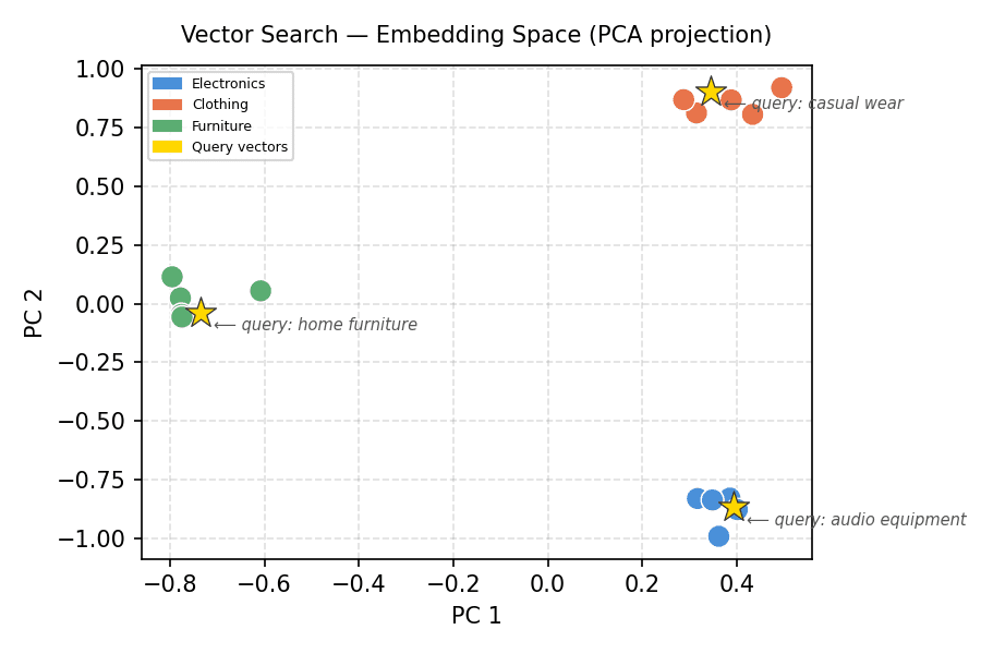
Embedding space, PCA projection. The clusters separate clearly, and each query vector lands inside the cluster it was generated from — the geometry that vector search relies on.
Visualising the similarity score distribution
For any given query it is useful to see how similarity scores are distributed across the whole index, not just within the top-k. This reveals whether the top result is a clear winner or only marginally better than everything else.
q_vec_furniture = queries("home furniture")
q_norm_furniture = normalize(q_vec_furniture.reshape(1, -1))
all_scores_furniture = (index.vectors @ q_norm_furniture.T).flatten()

sorted_idx_furniture = np.argsort(all_scores_furniture)(::-1)
sorted_scores_furniture = all_scores_furniture(sorted_idx_furniture)
sorted_labels_furniture = (products(i)(:30) + "…" if len(products(i)) > 30
                           else products(i) for i in sorted_idx_furniture)

# Define bar colors: green for furniture items, gray for others
bar_colors_furniture = ()
for i in sorted_idx_furniture:
    if i >= 10 and i <= 14:  # Furniture items are originally at indices 10-14
        bar_colors_furniture.append("#5BAD72") # Green for furniture
    else:
        bar_colors_furniture.append("#cccccc") # Gray for others

fig, ax = plt.subplots(figsize=(10, 5))
bars = ax.barh(sorted_labels_furniture(::-1), sorted_scores_furniture(::-1),
               color=bar_colors_furniture(::-1), edgecolor="white", height=0.65)

ax.axvline(sorted_scores_furniture(2), color="#5BAD72", linestyle="--",
           linewidth=1.2, label="Top-3 cutoff")
ax.set_xlim(sorted_scores_furniture.min() - 0.002, 1.001)
ax.set_xlabel("Cosine Similarity Score")
ax.set_title("Query: 'home furniture' — Similarity Across All Products", fontsize=11, pad=12)
ax.legend(fontsize=8)
ax.grid(axis="x", linestyle="--", alpha=0.4)
plt.tight_layout()
plt.savefig("score_distribution_furniture.png", dpi=150)
plt.show()
Output:
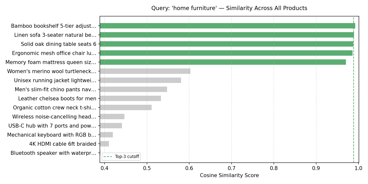
There is a clear separation between the relevant cluster and everything else. In practice this gap can be used to set a similarity threshold below which results are suppressed entirely.
Wrapping up
In roughly fifty lines of NumPy, the example assembles a working vector search engine: an index class that normalises and stores embeddings, a search method that uses matrix multiplication to compute cosine similarity, and two visualisations that expose the geometry behind the results. The natural next step is to replace the simulated embeddings with real ones — for instance by loading a sentence-transformer model and embedding an actual text corpus — and the index code above continues to work unchanged.
Limitations and what to watch
This implementation is intended for learning rather than production. A brute-force dot product compares the query against every stored vector, which is fine for a few dozen items but scales linearly with the size of the index; real systems with millions of vectors rely on approximate-nearest-neighbour structures such as HNSW or IVF, and on dedicated vector databases, to keep latency manageable. The example also uses simulated embeddings with an artificial cluster structure, so the clean separation shown here is easier than results on real, noisy text data.
Other practical concerns include the choice and quality of the embedding model, which determines whether semantic proximity actually reflects meaning; the cost of recomputing or updating embeddings as content changes; and the need for filtering, metadata and thresholding in a usable product. The core idea demonstrated here — normalise, take dot products, rank — remains the foundation, but a production deployment layers indexing, storage and evaluation on top of it. Readers interested in the broader tooling around AI systems may find the related overview of AI tool registries useful for context.
