
: Explained with an Example")
Dimensionality reduction techniques like PCA work wonderfully when datasets are linearly separable – but they break down when non-linear patterns appear. This is exactly what happens with datasets like two moons: PCA flattens the structure and merges classes together.
Kernel PCA corrects this limitation by mapping the data into a higher-dimensional feature space where nonlinear patterns are linearly separated. In this article, we will look at how kernel PCA works and will use a simple example to compare PCA vs kernel PCA, showing how a nonlinear dataset that PCA fails to separate becomes completely separable after applying kernel PCA.
Principal component analysis (PCA) is a linear dimensionality-reduction technique that identifies the directions (principal components) along which data vary most. It works by computing orthogonal linear combinations of the original features and interpolating the dataset onto directions of maximum variation.
These components are unrelated and arranged so that the first few capture most of the information in the data. PCA is powerful, but it comes with an important limitation: it can only highlight linear relationships in the data. When applied to non-linear datasets – such as the “two moons” example – it often fails to isolate the underlying structure.
Kernel PCA extends PCA to handle non-linear relationships. Instead of directly applying PCA to the original feature space, kernel PCA first uses a kernel function (such as RBF, polynomial, or sigmoid) to project the data into a higher-dimensional feature space where the nonlinear structure is linearly separated.
PCA is performed in this transformed space using a kernel matrix, without explicitly computing the higher-dimensional projection. This “kernel trick” allows kernel PCA to capture complex patterns that standard PCA cannot.

Now we will create a dataset that is nonlinear and then apply PCA on the dataset.
prepare dataset
We create a nonlinear “two moons” dataset using make_moons, which is ideal for demonstrating why PCA fails and why kernel PCA succeeds.
import matplotlib.pyplot as plt
from sklearn.datasets import make_moons

X, y = make_moons(n_samples=1000, noise=0.02, random_state=123)

plt.scatter(X(:, 0), X(:, 1), c=y)
plt.show()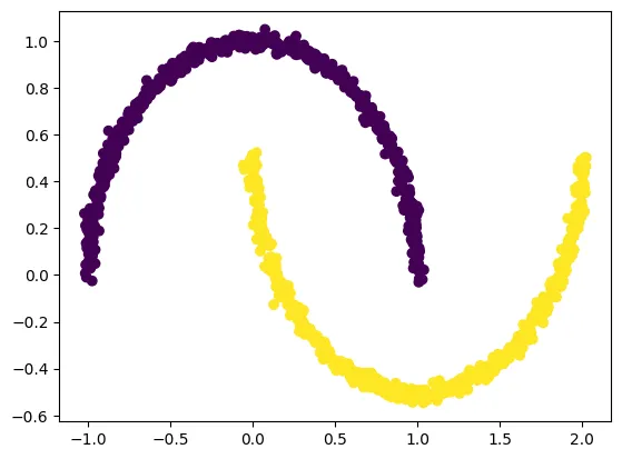
Applying PCA to dataset
from sklearn.decomposition import PCA
pca = PCA(n_components=2)
X_pca = pca.fit_transform(X)

plt.title("PCA")
plt.scatter(X_pca(:, 0), X_pca(:, 1), c=y)
plt.xlabel("Component 1")
plt.ylabel("Component 2")
plt.show()
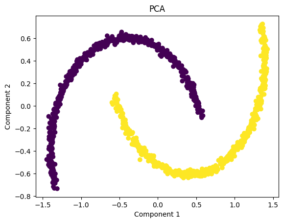
PCA visualization shows that the two moon-shaped clusters are interconnected even after dimension reduction. This occurs because PCA is a strictly linear technique – it can only rotate, scale, or flatten the data in direct directions of maximum variance.
Since the “two moons” dataset has a non-linear structure, PCA is unable to separate orbits or resolve curved shapes. As a result, the transformed data still looks almost identical to the original pattern, and both classes remain overlapped in the projected space.
Applying Kernel PCA on a Dataset
We now apply kernel PCA using the RBF kernel, which maps nonlinear data into a higher-dimensional space where it is linearly separable. The two classes in our dataset are linearly separable in kernel space. Kernel PCA uses a kernel function to project the dataset into a higher-dimensional space, where it is linearly separable.
from sklearn.decomposition import KernelPCA
kpca = KernelPCA(kernel="rbf", gamma=15)
X_kpca = kpca.fit_transform(X)

plt.title("Kernel PCA")
plt.scatter(X_kpca(:, 0), X_kpca(:, 1), c=y)
plt.show()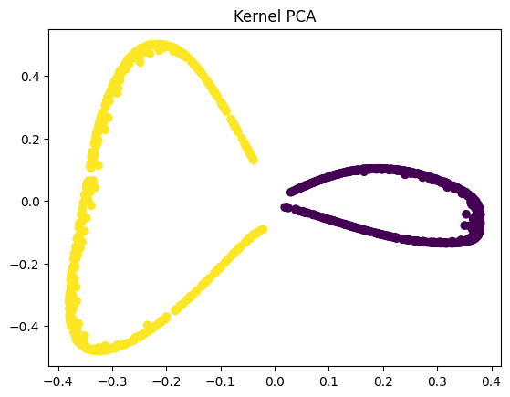
The goal of PCA (and dimensionality reduction in general) is not simply to compress the data – it is to reveal the underlying structure in a way that preserves meaningful variation. In nonlinear datasets such as the two-moon example, traditional PCA cannot “reveal” curved shapes because it only applies linear transformations.
However, kernel PCA performs a nonlinear mapping before applying PCA, allowing the algorithm to separate the moons into two clearly distinct groups. This separation is valuable because it makes downstream tasks like visualization, clustering, and even classification far more effective. When the data is linearly separable after transformation, simple models – such as linear classifiers – can successfully distinguish between classes, something that would be impossible in the original or PCA-transformed space.
While kernel PCA is powerful for handling nonlinear datasets, it comes with several practical challenges. The biggest drawback is computational cost – because it relies on calculating pairwise similarity between all data points, the algorithm has O(n²) Time and memory complexity makes it slow and memory-heavy for large datasets.
Another challenge is model selection: choosing the right kernel (RBF, polynomial, etc.) and tuning parameters such as gamma can be difficult and often requires experimentation or domain expertise.
Kernel PCA can also be difficult to interpret, because the transformed components no longer correspond to intuitive directions in the original feature space. Finally, it is sensitive to missing values and outliers, which can distort the kernel matrix and degrade performance.
check it out full code hereFeel free to check us out GitHub page for tutorials, code, and notebooksAlso, feel free to follow us Twitter And don’t forget to join us 100k+ ml subreddit and subscribe our newsletterwait! Are you on Telegram? Now you can also connect with us on Telegram.

I am a Civil Engineering graduate (2022) from Jamia Millia Islamia, New Delhi, and I have a keen interest in Data Science, especially Neural Networks and their application in various fields.