

In deep learning, classification models don’t just need to make predictions – they need to express confidence. This is where the softmax activation function comes in. Softmax takes the raw, unscaled scores produced by a neural network and transforms them into a well-defined probability distribution, making it possible to interpret each output as the probability of a specific class.
This property makes softmax the cornerstone of multi-class classification tasks from image recognition to language modeling. In this article, we will develop an intuitive understanding of how softmax works and why its implementation details are more important than they first appear. check it out full code here,
Implementation of Naive Softmax
import torch

def softmax_naive(logits):
    exp_logits = torch.exp(logits)
    return exp_logits / exp_logits.sum(dim=1, keepdim=True)
This function implements softmax activation in its simplest form. It exponentiates each logit and normalizes it by summing all exponential values across all classes, generating a probability distribution for each input sample.
Although this implementation is mathematically correct and easy to read, it is numerically unstable – large positive logs can cause overflow, and large negative logs can cause underflow to zero. As a result, this version should be avoided in real training pipelines. check it out full code here,
Sample Logit and Target Labels
This example defines a small batch with three samples and three classes to represent both normal and failure cases. The first and third samples have reasonable logit values and behave as expected during softmax calculations. The second sample deliberately includes extreme values (1000 and -1000) to demonstrate numerical instability – this is where the simple softmax implementation fails.
The target tensor specifies the correct class index for each sample and will be used to calculate the classification loss and see how instability is propagated during backpropagation. check it out full code here,
# Batch of 3 samples, 3 classes
logits = torch.tensor((
    (2.0, 1.0, 0.1),
    (1000.0, 1.0, -1000.0),
    (3.0, 2.0, 1.0)
), requires_grad=True)

targets = torch.tensor((0, 2, 1))
Forward Pass: Softmax Output and Failure Case
During the forward pass, a naive softmax function is applied to the logits to generate class probabilities. For normal logit values (first and third samples), the output is a valid probability distribution where the values lie between 0 and 1 and sum to 1.
However, the second sample clearly highlights the numerical issue: exponentiation of 1000 overflows. infiniteWhile -1000 is underflow ZeroThis results in invalid operations during normalization, producing NaN values and zero probabilities, Once Nan Appearing at this stage, it corrupts all subsequent calculations, rendering the model useless for training. check it out full code here,
# Forward pass
probs = softmax_naive(logits)

print("Softmax probabilities:")
print(probs)
Goal Probabilities and Loss Details
Here, we extract the predicted probability corresponding to the true class for each sample. While the first and third samples return valid probabilities, the target probability of the second sample is 0.0, caused by numerical underflow in the softmax calculation. When loss is calculated using -log(p)Taking the logarithm of 0.0 gives the result +,
This makes the overall loss infinite, which is a serious failure during training. Once the loss becomes infinite, the sequential computation becomes unstable, leading to eyes Effectively preventing further learning during backpropagation. check it out full code here,
# Extract target probabilities
target_probs = probs(torch.arange(len(targets)), targets)

print("nTarget probabilities:")
print(target_probs)

# Compute loss
loss = -torch.log(target_probs).mean()
print("nLoss:", loss)
Backpropagation: gradual corruption
When backpropagation begins, the effect of infinite loss becomes immediately visible. The gradients for the first and third samples remain limited because their softmax outputs were well-behaved. However, the second sample loss produces NaN gradients in all classes due to the log(0) operation.
These NaNs propagate backward through the network, corrupting the weight updates and effectively breaking the training. This is why numerical instability at the softmax-loss threshold is so dangerous – once NaNs appear, recovery is almost impossible without restarting training. check it out full code here,
loss.backward()

print("nGradients:")
print(logits.grad)
Numerical instability and its consequences
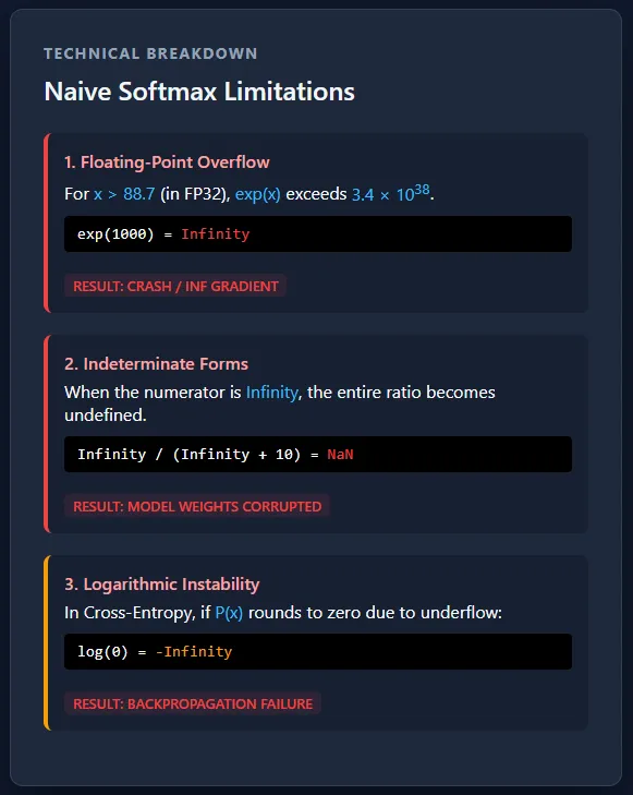
Separating softmax and cross-entropy creates a serious numerical stability risk due to exponential overflow and underflow. Large logs can push the probabilities to infinity or zero, leading to log(0) and NaN gradients that quickly corrupt the training. At production scale, this is not a rare edge case, but a certainty – without stable, connected implementations, large multi-GPU training runs will fail unexpectedly.
The main numerical problem comes from the fact that computers cannot represent infinitely large or infinitely small numbers. Floating-point formats like FP32 have strict limits on how large or small a value can be stored. When softmax computes exp(x), large positive values grow so quickly that they exceed the maximum representable number and turn to infinity, while large negative values shrink so much that they approach zero. Once a value reaches infinity or zero, subsequent operations such as division or logarithms break down and produce invalid results. check it out full code here,
Implementing static cross-entropy loss using LogSumExp
This implementation calculates the cross-entropy loss directly from the raw log without explicitly calculating the softmax probabilities. To maintain numerical consistency, the log is shifted first by subtracting the maximum value per sample, ensuring that the exponents remain within safe limits.
The LogSumExp trick is then used to calculate the normalization term, after which the original (unshifted) target logit is subtracted to obtain the true loss. This approach avoids overflow, underflow, and NaN gradients, and demonstrates how cross-entropy is implemented in a production-grade deep learning framework. check it out full code here,
def stable_cross_entropy(logits, targets):

    # Find max logit per sample
    max_logits, _ = torch.max(logits, dim=1, keepdim=True)

    # Shift logits for numerical stability
    shifted_logits = logits - max_logits

    # Compute LogSumExp
    log_sum_exp = torch.log(torch.sum(torch.exp(shifted_logits), dim=1)) + max_logits.squeeze(1)

    # Compute loss using ORIGINAL logits
    loss = log_sum_exp - logits(torch.arange(len(targets)), targets)

    return loss.mean()
Steady forward and backward pass
Running the stable cross-entropy implementation on the same extreme logs produces a finite loss and well-defined gradients. Even if a sample contains very large values (1000 and -1000), the LogSumExp formulation keeps all intermediate counts within a safe numerical range. As a result, backpropagation completes successfully without generating NaNs, and each class receives a meaningful gradient signal.
This confirms that the previously observed instability was not due to the data, but to naive separation of softmax and cross-entropy – a problem that was completely solved using numerically stable, fused loss formulations. check it out full code here,
logits = torch.tensor((
    (2.0, 1.0, 0.1),
    (1000.0, 1.0, -1000.0),
    (3.0, 2.0, 1.0)
), requires_grad=True)

targets = torch.tensor((0, 2, 1))

loss = stable_cross_entropy(logits, targets)
print("Stable loss:", loss)

loss.backward()
print("nGradients:")
print(logits.grad)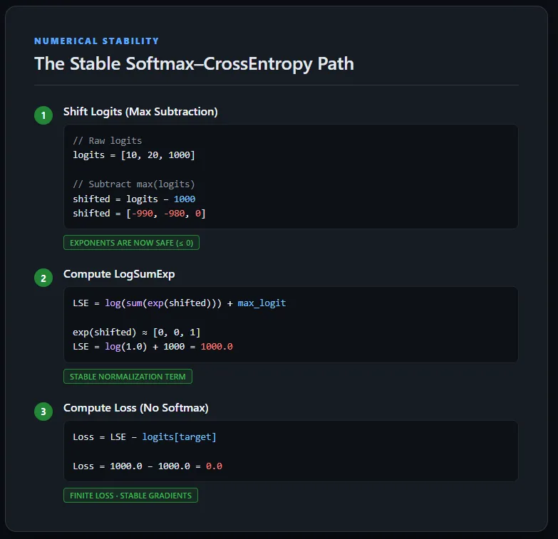
conclusion
In practice, the gap between mathematical formulas and real-world code is where many training failures arise. While softmax and cross-entropy are mathematically well-defined, their naive implementation ignores the limited precision limits of IEEE 754 hardware, making underflow and overflow inevitable.
The main solution is simple but important: log shift before the exponential and work in the log domain whenever possible. Most importantly, training rarely requires categorical probabilities – stable log-likelihoods are sufficient and much safer. When the output loss suddenly turns to NaN, it is often a sign that the softmax is being calculated manually when it should not be.
check it out full code hereAlso, feel free to follow us Twitter And don’t forget to join us 100k+ ml subreddit and subscribe our newsletterwait! Are you on Telegram? Now you can also connect with us on Telegram.
Check out our latest releases ai2025.devA 2025-focused analytics platform that models launches, benchmarks and transforms ecosystem activity into a structured dataset that you can filter, compare and export

I am a Civil Engineering graduate (2022) from Jamia Millia Islamia, New Delhi, and I have a keen interest in Data Science, especially Neural Networks and their application in various fields.