

Topic modeling uncovers hidden themes in large document collections. Traditional methods such as Latent Dirichlet Allocation (LDA) rely on word frequency and treat text as a bag of words, which often misses deeper context and meaning. BERTopic takes a different approach, combining transformer embeddings, clustering, and a class-based TF-IDF (c-TF-IDF) weighting to capture the semantic relationships between documents and produce more meaningful, context-aware topics. This article explains how modern topic modeling in Python works with BERTopic and walks through a step-by-step implementation.
What is BERTopic?
BERTopic is a modular topic modeling framework that treats topic discovery as a pipeline of independent but connected steps, combining deep learning with classical natural language processing to produce coherent, explainable topics. The core idea is to transform documents into semantic embeddings, cluster them by similarity, and then extract representative words for each cluster.
Key components of the BERTopic pipeline
1. Preprocessing
The first step prepares the raw text. Unlike traditional NLP pipelines, BERTopic does not require heavy preprocessing; minimal cleanup, such as lowercasing, removing extra spaces, and filtering out very short documents, is usually sufficient.
2. Document embedding
Each document is converted into a dense vector using a transformer-based model such as Sentence-Transformers, which lets the model capture semantic relationships between documents. Expressed mathematically:
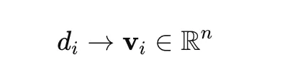
where d is a document and v its vector representation.
3. Dimensionality reduction
High-dimensional embeddings are hard to cluster effectively, so BERTopic uses UMAP to reduce dimensionality while preserving the structure of the data.
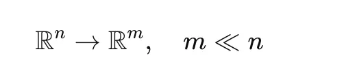
This step improves both clustering performance and computational efficiency.
4. Clustering
After dimensionality reduction, clustering is performed with HDBSCAN, a density-based algorithm that does not require the number of clusters to be set in advance. Documents that do not fit any cluster confidently are labelled -1 and treated as outliers.

5. c-TF-IDF topic representation
Once clusters are formed, BERTopic derives topic representations using c-TF-IDF, computed from a term-frequency component, an inverse-document-frequency component, and their combination:
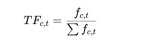
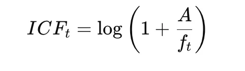

This highlights words that are distinctive within a cluster while downplaying words common across clusters.
Hands-on implementation
The following walkthrough demonstrates a minimal BERTopic implementation on a very small dataset. The aim is not a production-grade model but a clear view of how the pipeline fits together: preprocessing the text, configuring UMAP and HDBSCAN, training the model, and inspecting the topics.
Step 1: Import the libraries and prepare the dataset
The required libraries are imported first. The re module handles basic text preprocessing, while UMAP and HDBSCAN provide dimensionality reduction and clustering, and BERTopic ties the components into a pipeline. A short list of sample documents spanning distinct themes, such as space and philosophy, is created to show how BERTopic separates text into topics.
import re
import umap
import hdbscan
from bertopic import BERTopic

docs = (
"NASA launched a satellite",
"Philosophy and religion are related",
"Space exploration is growing"
)
Step 2: Preprocess the text
This step applies basic cleaning. Each document is lowercased so that, for example, different casings of the same word are treated as one token, and extra spaces are removed to standardise formatting. Even though transformer embeddings rely less on heavy cleaning, light normalisation reduces noise in the input.
def preprocess(text):
    text = text.lower()
    text = re.sub(r"s+", " ", text)
    return text.strip()

docs = (preprocess(doc) for doc in docs)
Step 3: Configure UMAP
UMAP reduces the dimensionality of the document embeddings before clustering, projecting them into a lower-dimensional space while preserving semantic relationships. The setting init="random" matters here because the dataset is tiny: with only a few documents, UMAP’s default spectral initialisation can fail, so random initialisation avoids that error. The values n_neighbors=2 and n_components=2 are chosen to suit the small dataset.
umap_model = umap.UMAP(
    n_neighbors=2,
    n_components=2,
    min_dist=0.0,
    metric="cosine",
    random_state=42,
    init="random"
)
Step 4: Configure HDBSCAN
HDBSCAN groups similar documents after dimensionality reduction and, unlike K-means, does not require the number of clusters in advance. Here min_cluster_size=2 means at least two documents are needed to form a cluster.
hdbscan_model = hdbscan.HDBSCAN(
    min_cluster_size=2,
    metric="euclidean",
    cluster_selection_method="eom",
    prediction_data=True
)
Step 5: Create the BERTopic model
The model is built by passing the custom UMAP and HDBSCAN configurations, reflecting BERTopic’s modularity: individual components can be swapped or tuned for the dataset and use case. Enabling probability calculation lets the model estimate topic probabilities per document, and verbose output is useful during experimentation because it shows progress and internal steps.
topic_model = BERTopic(
    umap_model=umap_model,
    hdbscan_model=hdbscan_model,
    calculate_probabilities=True,
    verbose=True
)
Step 6: Fit the model
This is the main training phase, in which BERTopic runs the full pipeline internally: converting documents to embeddings, reducing their dimensions with UMAP, clustering them with HDBSCAN, and extracting topic words with c-TF-IDF. The result is stored as the topic label assigned to each document and the associated probability distribution.
topics, probs = topic_model.fit_transform(docs) Step 7: Inspect topic assignments and information
The final step examines the model’s output. Printing the topics shows the label assigned to each document; get_topic_info() displays a summary table of all topics with their IDs and document counts; and get_topic(topic_id) returns the most representative words for a topic. Filtering out the -1 label excludes outliers, documents not confidently assigned to any cluster, which is normal behaviour for density-based clustering and prevents unrelated documents from being forced into a topic.
print("Topics:", topics)
print(topic_model.get_topic_info())

for topic_id in sorted(set(topics)):
    if topic_id != -1:
        print(f"nTopic {topic_id}:")
        print(topic_model.get_topic(topic_id))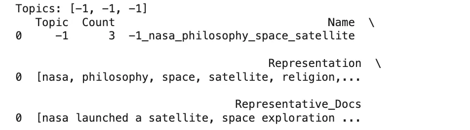
Benefits of BERTopic
BERTopic’s main strengths follow from its design. It captures semantic meaning through transformer embeddings rather than raw word frequency, so it groups documents by context. It detects the number of topics automatically via HDBSCAN, removing the need to guess that number up front. It is modular, allowing each stage to be customised, and its c-TF-IDF representations make topics relatively interpretable.
Limitations and what to watch
BERTopic is more computationally demanding than frequency-based methods, mainly because generating embeddings is expensive, which matters for large datasets and may call for a GPU or a lighter embedding model. Results depend on the chosen embedding model and on UMAP and HDBSCAN settings, so small parameter changes can shift the topics, and very small datasets (as in this demo) behave differently from realistic corpora. Density-based clustering can also assign many documents to the outlier (-1) group, which may require tuning. As with any unsupervised method, topic labels still need human interpretation, and reproducibility requires fixing random seeds and pinning library versions. The official BERTopic documentation covers configuration options in depth.
Conclusion
BERTopic offers a modern, semantically aware approach to topic modeling that frequently produces more coherent and context-sensitive topics than bag-of-words methods. Its modular pipeline, embeddings, dimensionality reduction, clustering, and c-TF-IDF, makes it adaptable to many text-analysis tasks while keeping the results interpretable. A related applied example appears in the guide to analysing customer call recordings.
Frequently asked questions
How does BERTopic differ from traditional topic modeling such as LDA? It uses semantic embeddings rather than word frequency, allowing it to capture context and meaning more effectively.
Does BERTopic require specifying the number of topics? No. It uses HDBSCAN clustering, which automatically detects the natural number of topics without a predefined count.
What is a key limitation of BERTopic? It is computationally expensive because of embedding generation, especially on large datasets.
